Demonstration 3: Multiomics (scRNA-seq + scATAC-seq) Simulation Evaluation

Introduction

Single-cell multiomics technologies allow simultaneous or parallel measurement of multiple cellular features — most commonly gene expression (scRNA-seq) and chromatin accessibility (scATAC-seq). Simulating multiomics data presents unique challenges because algorithms must preserve not only the distinct statistical properties of each individual modality, but also the biological coupling and regulatory relationships between them.

scSimEval is designed to evaluate simulation fidelity across three distinct multiomics experimental designs, each with a different level of cell-level pairing between modalities. Understanding which design your simulated data belongs to is essential for selecting the correct evaluation functions.

Part 1: Understanding Multiomics Data Types

1.1 Paired Multiomics (Co-assay)

Definition: Both scRNA-seq and scATAC-seq are measured simultaneously from the exact same individual cells. Each cell barcode in the RNA matrix has a corresponding and biologically meaningful entry at the same column index in the ATAC matrix.

Technologies: 10x Chromium Multiome, SHARE-seq, SNARE-seq, Paired-seq, ASTAR-seq

Simulators: scMultiSim (Li et al., Nat Methods 2023), SymSim2+ATAC, MultiSim

What scSimEval can evaluate:

✅ Full unimodal evaluation for each modality (Categories 1–6 and 8)
✅ All Category 7 cross-modal coupling metrics:
- FOSCTTM and Match@1 (cell alignment in joint embedding space)
- Cross-modal generation fidelity (predict ATAC from RNA, or vice versa)
- Direct peak-to-gene regulatory linkage (promoter/enhancer accessibility vs. transcription)
- Cross-modality feature correlation fidelity
- Modality alignment and mixing score in joint latent space

1.2 Unpaired Multiomics (Independent profiling)

Definition: scRNA-seq and scATAC-seq are profiled from different cells derived from the same biological tissue, cell line, or sample. Cell barcodes do not correspond between modalities — column i of the RNA matrix and column i of the ATAC matrix represent entirely different cells.

Technologies: Bulk ATAC + scRNA-seq, independent 10x scATAC + scRNA experiments on the same tissue, sci-ATAC-seq paired with scRNA-seq on sibling aliquots

Simulators: Splatter (RNA only) + ArchR (ATAC only) used separately, AMULET

What scSimEval can evaluate:

✅ Full unimodal evaluation for each modality independently (Categories 1–6 and 8)
✅ Population-level cross-modal metrics that do not require cell-by-cell pairing:
- Cross-modal label transfer accuracy (evaluate_cross_modal_prediction)
- Co-expression module fidelity (calc_coexpression_module_fidelity)
- Peak co-accessibility fidelity (calc_peak_coaccessibility_fidelity)
- Network topology similarity (calc_network_jaccard)
- Chromatin accessibility profile concordance (calc_accessibility_profile_concordance)
❌ NOT applicable (require 1-to-1 cell pairing):
- FOSCTTM and Match@1 (calc_foscttm)
- Cross-modal generation fidelity (calc_cross_modal_generation)
- Peak-to-gene regulatory coupling (calc_atac_rna_coupling)
- Cross-modality correlation (calc_cross_modality_correlation)

Note: Using evaluate_multiomics_accuracy() directly on unpaired data is NOT recommended because it internally calls paired metrics. Instead, use evaluate_simulation_accuracy() per modality plus the population-level functions listed above, and combine results with evaluate_multiple_datasets().

1.3 Mosaic Multiomics (Partial co-measurement)

Definition: A subset of cells has measurements in both modalities, while the remaining cells have measurements in only one modality. This arises from experimental designs that pool paired and unpaired samples, or from modality dropout in co-assay experiments.

Technologies: DOGMA-seq (DNA + RNA + protein + ATAC, but with high dropout), mosaic pooling designs (mixing Multiome cells with scRNA-only or scATAC-only cells), partially overlapping patient cohorts

Simulators: MultiVI (Lopez et al., Nat Methods 2023), Cobolt, MOFA+ imputation

What scSimEval can evaluate:

✅ Full unimodal evaluation on the complete single-modality matrices (Categories 1–6, 8)
✅ Paired Category 7 coupling metrics on the co-assayed cell subset only
✅ Population-level cross-modal metrics on the full matrices
⚠️ Recommendation: Extract the co-assayed subset first, then call paired metrics on it

1.4 Metric Compatibility Summary

Metric / Function	Paired	Unpaired	Mosaic (paired subset)
`evaluate_simulation_accuracy()` per modality	✅	✅	✅
`evaluate_clustering_metrics()`	✅	✅	✅
`evaluate_batch_metrics()`	✅	✅	✅
`evaluate_deg_fidelity()`	✅	✅	✅
`evaluate_trajectory_metrics()`	✅	✅	✅
`calc_coexpression_module_fidelity()`	✅	✅	✅
`calc_peak_coaccessibility_fidelity()`	✅	✅	✅
`calc_accessibility_profile_concordance()`	✅	✅	✅
`calc_network_jaccard()`	✅	✅	✅
`evaluate_cross_modal_prediction()`	✅	✅	✅
`calc_modality_alignment()`	✅	⚠️ needs integration first	✅ on subset
`calc_foscttm()`	✅	❌	✅ on subset
`calc_cross_modal_generation()`	✅	❌	✅ on subset
`calc_atac_rna_coupling()`	✅	❌	✅ on subset
`calc_cross_modality_correlation()`	✅	❌	✅ on subset
`evaluate_multiomics_accuracy()`	✅	❌ direct use	✅ on subset

Part 2: Evaluating Paired Multiomics

2.1 Loading the Example Paired Dataset

scSimEval includes a paired scRNA-seq + scATAC-seq dataset (example_multiomics) where every column in the RNA matrix corresponds to the same cell in the ATAC matrix:

library(scSimEval)

# Load packaged paired multiomics example dataset
data(example_multiomics)

cat("Reference RNA dimensions:", dim(example_multiomics$ref_multi$rna), "\n")
#> Reference RNA dimensions: 60 80
cat("Reference ATAC dimensions:", dim(example_multiomics$ref_multi$atac), "\n")
#> Reference ATAC dimensions: 60 80
cat("Simulated RNA dimensions:", dim(example_multiomics$sim_multi$rna), "\n")
#> Simulated RNA dimensions: 60 80
cat("Simulated ATAC dimensions:", dim(example_multiomics$sim_multi$atac), "\n")
#> Simulated ATAC dimensions: 60 80
cat("Cell types:", levels(example_multiomics$cell_types), "\n")
#> Cell types: TypeA TypeB

The dataset contains:

ref_multi: Named list rna (count matrix) and atac (peak accessibility matrix), both measured from the same cells.
sim_multi: Simulated paired rna and atac matrices.
cell_types: Cell type annotations shared across both modalities.
batch_info: Batch labels shared across both modalities.
resource_stats: Hardware logs (runtime in seconds and peak RAM in MiB).

2.2 Alignment in Joint Embedding Space (FOSCTTM & Match@1)

FOSCTTM (Fraction Of Samples Closer Than The True Match) quantifies whether paired cells are each other’s nearest neighbors in joint latent space. Valid only for paired data.

# Compute reduced representations (PCA) for RNA and ATAC
pca_rna  <- prcomp(t(example_multiomics$ref_multi$rna), rank. = 5)$x
pca_atac <- prcomp(t(example_multiomics$ref_multi$atac), rank. = 5)$x

foscttm_res <- calc_foscttm(x = pca_rna, y = pca_atac)

cat("Bidirectional FOSCTTM score:", round(foscttm_res$foscttm, 4), "\n")
#> Bidirectional FOSCTTM score: 0.455
cat("Top-1 Match Rate (Match@1):", round(foscttm_res$match_at_1, 4), "\n")
#> Top-1 Match Rate (Match@1): 0.0125

A score of 0.00 indicates perfect alignment; 0.50 represents random chance.

Tests whether chromatin accessibility profiles in simulated ATAC can predict cell types annotated in RNA. This metric works for all three data types because it uses population-level kNN classification:

transfer_res <- evaluate_cross_modal_prediction(
  mod1_data  = example_multiomics$sim_multi$atac,
  cell_types = example_multiomics$cell_types
)

cat("Cross-Modal Prediction Accuracy:", round(transfer_res$cross_modal_accuracy, 4), "\n")
#> Cross-Modal Prediction Accuracy: 0.8125
cat("Cross-Modal Macro F1 Score:", round(transfer_res$cross_modal_F1, 4), "\n")
#> Cross-Modal Macro F1 Score: 0.8057

2.4 Master Paired Pipeline: `evaluate_multiomics_accuracy()`

For fully paired data, the master function coordinates all 8 categories:

master_eval <- evaluate_multiomics_accuracy(
  ref_multi  = example_multiomics$ref_multi,
  sim_multi  = example_multiomics$sim_multi,
  cell_types = example_multiomics$cell_types,
  elapsed_time = example_multiomics$resource_stats$elapsed_time,
  memory_mb    = example_multiomics$resource_stats$memory_mb,
  verbose      = FALSE
)

head(master_eval$benchmark_summary_table)
#>                    Category     Property        Metric        Value Modality
#> 1 Distributional Properties library_size           MAD 1.500000e+01      rna
#> 2 Distributional Properties library_size            KS 2.125000e-01      rna
#> 3 Distributional Properties library_size           MAE 1.506250e+01      rna
#> 4 Distributional Properties library_size          RMSE 1.571504e+01      rna
#> 5 Distributional Properties library_size            OV 8.370258e-01      rna
#> 6 Distributional Properties library_size Bhattacharyya 1.188839e-04      rna

Part 3: Evaluating Unpaired Multiomics

For unpaired data, scRNA-seq and scATAC-seq come from different cells. The recommended workflow is to evaluate each modality independently and combine results.

3.1 Step-by-Step Workflow for Unpaired Data

library(scSimEval)
data(example_scrna)   # RNA modality
data(example_scatac)  # ATAC modality (different cells)

# ── Step 1: Evaluate each modality independently ──────────────────────────────
rna_eval <- evaluate_simulation_accuracy(
  ref_data = example_scrna$ref,
  sim_data = example_scrna$sim,
  compute_bivariate = FALSE,
  verbose = FALSE
)

atac_eval <- evaluate_simulation_accuracy(
  ref_data = example_scatac$ref,
  sim_data = example_scatac$sim,
  compute_bivariate = FALSE,
  verbose = FALSE
)

# ── Step 2: Population-level cross-modal metrics (no cell pairing needed) ─────

# 2a. Co-expression module fidelity (RNA only, no pairing needed)
module_fid <- calc_coexpression_module_fidelity(
  ref_mat = example_scrna$ref,
  sim_mat = example_scrna$sim
)
cat("Module correlation r:", round(module_fid$module_correlation_r, 4), "\n")

# 2b. Peak co-accessibility fidelity (ATAC only, no pairing needed)
coaccess_fid <- calc_peak_coaccessibility_fidelity(
  ref_atac = example_scatac$ref,
  sim_atac = example_scatac$sim
)
cat("RV coefficient:", round(coaccess_fid$rv_coefficient, 4), "\n")

# 2c. Cross-modal label transfer (uses ATAC features to predict RNA-based labels)
# NOTE: cell_types come from the RNA experiment; applied to ATAC data for transfer
label_transfer <- evaluate_cross_modal_prediction(
  mod1_data  = example_scatac$sim,
  cell_types = example_scatac$cell_types
)
cat("Label transfer accuracy:", round(label_transfer$cross_modal_accuracy, 4), "\n")

# ── Step 3: Consolidate and compare across modalities ─────────────────────────
dataset_collection <- list(
  "Method_A-RNA"  = list(ref = example_scrna$ref,  sim = example_scrna$sim),
  "Method_A-ATAC" = list(ref = example_scatac$ref, sim = example_scatac$sim)
)

consolidated <- evaluate_multiple_datasets(
  datasets          = dataset_collection,
  pair_by_prefix    = TRUE,
  compute_bivariate = FALSE,
  verbose           = FALSE
)

print(consolidated$dataset_overview)

Key point: Do NOT call calc_foscttm(), calc_cross_modal_generation(), calc_atac_rna_coupling(), or calc_cross_modality_correlation() on unpaired data. These functions assume row/column i of the RNA matrix matches row/column i of the ATAC matrix — an assumption that is biologically false for unpaired experiments.

Part 4: Evaluating Mosaic Multiomics

For mosaic data (where only some cells have both modalities), the strategy is:

Extract co-assayed cells — the subset that has measurements in both RNA and ATAC.
Run paired metrics on this subset using evaluate_multiomics_accuracy() or individual Category 7 functions.
Run unimodal metrics on the full single-modality matrices.

4.1 Step-by-Step Workflow for Mosaic Data

# Suppose your mosaic simulator output looks like this:
# - sim_rna_full: RNA matrix for ALL cells (including RNA-only cells)
# - sim_atac_full: ATAC matrix for ALL cells (including ATAC-only cells)
# - paired_cell_idx: logical or integer index of cells with BOTH modalities

# ── Step 1: Identify co-assayed cell subset ───────────────────────────────────
# (This index should come from your simulator's output metadata)
# Example: first 200 cells are co-assayed, rest are single-modality
paired_idx   <- 1:200

sim_rna_paired  <- sim_rna_full[, paired_idx]
sim_atac_paired <- sim_atac_full[, paired_idx]
ref_rna_paired  <- ref_rna_full[, paired_idx]
ref_atac_paired <- ref_atac_full[, paired_idx]

# ── Step 2: Paired coupling metrics on the co-assayed subset ──────────────────
paired_eval <- evaluate_multiomics_accuracy(
  ref_multi  = list(rna = ref_rna_paired, atac = ref_atac_paired),
  sim_multi  = list(rna = sim_rna_paired, atac = sim_atac_paired),
  cell_types = cell_types_paired,
  verbose    = FALSE
)

# ── Step 3: Full unimodal evaluation on the complete matrices ─────────────────
rna_full_eval <- evaluate_simulation_accuracy(
  ref_data = ref_rna_full,
  sim_data = sim_rna_full,
  compute_bivariate = FALSE,
  verbose = FALSE
)

atac_full_eval <- evaluate_simulation_accuracy(
  ref_data = ref_atac_full,
  sim_data = sim_atac_full,
  compute_bivariate = FALSE,
  verbose = FALSE
)

# ── Step 4: Population-level cross-modal metrics (full matrices) ──────────────
module_fid <- calc_coexpression_module_fidelity(ref_rna_full, sim_rna_full)
coaccess   <- calc_peak_coaccessibility_fidelity(ref_atac_full, sim_atac_full)

Part 5: Visualization

scSimEval visualization functions work seamlessly across unimodal, paired, and unpaired multiomics configurations:

# Multi-dataset consolidated benchmark bubble matrix
plot_benchmark_bubble_matrix(
  data  = consolidated,
  title = "Benchmarking Multiomics Simulators"
)

# Evaluation summary horizontal bar matrix
plot_evaluation_summary(
  data  = consolidated,
  title = "Multiomics Simulator Leaderboard"
)

5.1 Low-Dimensional Multiomics Cell Embeddings

To visually examine whether simulated cells maintain the biological manifold of empirical data across modalities, researchers can project reference and simulated cells into low-dimensional UMAP, t-SNE, or PCA coordinates:

# Compute low-dimensional embeddings for the scRNA-seq modality
emb_rna <- compute_dataset_embeddings(
  reference   = example_multiomics$ref_multi$rna,
  simulated   = list("Multi_Sim" = example_multiomics$sim_multi$rna),
  reduction   = "pca",
  n_pcs       = 5,
  cell_types  = example_multiomics$cell_types
)

# Plot multiomics cell embeddings
plot_dataset_embeddings(
  embedding_data = emb_rna,
  reduction      = "pca",
  layout         = "side_by_side",
  color_by       = "cell_type"
)


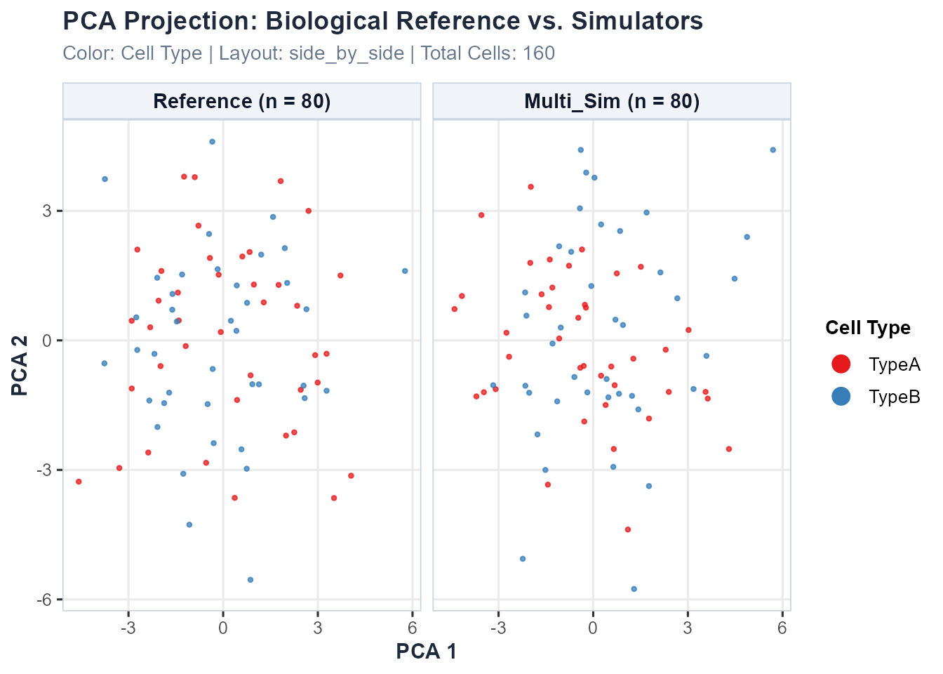
# Quantitative embedding quality metrics
knitr::kable(compute_embedding_quality_metrics(emb_rna), digits = 4)

Dataset	Role	Cells (N)	Mean Silhouette	ARI (Cluster Fidelity)	Mean Library Size	Mean Detected Features	Library Size Diff (%)
Reference	Reference	80	-0.0101	-0.0027	256.3	49.2	0.00
Multi_Sim	Simulated	80	0.0037	-0.0071	242.3	48.3	5.46

Part 6: Summary

Data Type	Example Technologies	`evaluate_multiomics_accuracy()`	Category 7 Metrics	Recommended Function
Paired	10x Multiome, SHARE-seq	✅ Direct	All 6 metrics	`evaluate_multiomics_accuracy()`
Unpaired	Independent scRNA + scATAC	❌ Not valid	Modularity, label transfer, network only	`evaluate_simulation_accuracy()` × 2 + `evaluate_multiple_datasets()`
Mosaic	DOGMA-seq, mosaic pooling	✅ On paired subset	All 6 metrics on paired subset	Subset first, then `evaluate_multiomics_accuracy()`

The most important rule: Cell-pairing metrics (FOSCTTM, cross-modal generation, peak-to-gene coupling) are only scientifically valid when the RNA and ATAC columns correspond to the same physical cells. For unpaired and mosaic data, rely on population-level metrics and per-modality unimodal evaluation.

sessionInfo()
#> R version 4.6.1 (2026-06-24 ucrt)
#> Platform: x86_64-w64-mingw32/x64
#> Running under: Windows 11 x64 (build 26200)
#> 
#> Matrix products: default
#>   LAPACK version 3.12.1
#> 
#> locale:
#> [1] LC_COLLATE=English_India.utf8  LC_CTYPE=English_India.utf8   
#> [3] LC_MONETARY=English_India.utf8 LC_NUMERIC=C                  
#> [5] LC_TIME=English_India.utf8    
#> 
#> time zone: Asia/Calcutta
#> tzcode source: internal
#> 
#> attached base packages:
#> [1] stats     graphics  grDevices utils     datasets  methods   base     
#> 
#> other attached packages:
#> [1] scSimEval_0.99.7
#> 
#> loaded via a namespace (and not attached):
#>   [1] RColorBrewer_1.1-3          jsonlite_2.0.0             
#>   [3] magrittr_2.0.5              modeltools_0.2-24          
#>   [5] farver_2.1.2                nloptr_2.2.1               
#>   [7] rmarkdown_2.32              provenance_4.4             
#>   [9] fs_2.1.0                    ragg_1.5.2                 
#>  [11] vctrs_0.7.3                 memoise_2.0.1              
#>  [13] minqa_1.2.8                 htmltools_0.5.9            
#>  [15] S4Arrays_1.13.0             curl_8.0.0                 
#>  [17] BiocNeighbors_2.7.3         SparseArray_1.13.2         
#>  [19] overlapping_2.5             sass_0.4.10                
#>  [21] bslib_0.12.0                htmlwidgets_1.6.4          
#>  [23] desc_1.4.3                  testthat_3.3.2             
#>  [25] httr2_1.3.0                 cachem_1.1.0               
#>  [27] igraph_2.3.3                lifecycle_1.0.5            
#>  [29] pkgconfig_2.0.3             Matrix_1.7-6               
#>  [31] R6_2.6.1                    fastmap_1.2.0              
#>  [33] clue_0.3-68                 rbibutils_2.4.1            
#>  [35] MatrixGenerics_1.25.0       digest_0.6.39              
#>  [37] S4Vectors_0.51.10           irlba_2.3.7                
#>  [39] IsoplotR_7.0                textshaping_1.0.5          
#>  [41] GenomicRanges_1.65.4        RSQLite_3.53.3             
#>  [43] labeling_0.4.3              philentropy_0.10.0         
#>  [45] filelock_1.0.3              abind_1.4-8                
#>  [47] compiler_4.6.1              proxy_0.4-29               
#>  [49] bit64_4.8.6                 withr_3.0.3                
#>  [51] S7_0.2.2                    BiocParallel_1.47.0        
#>  [53] DBI_1.3.0                   MASS_7.3-66                
#>  [55] DelayedArray_0.39.8         bluster_1.23.1             
#>  [57] tools_4.6.1                 otel_0.2.0                 
#>  [59] prabclus_2.3-5              nnet_7.3-21                
#>  [61] glue_1.8.1                  nlme_3.1-171               
#>  [63] grid_4.6.1                  waddR_1.27.0               
#>  [65] cluster_2.1.8.3             ade4_1.7-24                
#>  [67] generics_0.1.4              gtable_0.3.6               
#>  [69] class_7.3-24                XVector_0.52.0             
#>  [71] flexmix_2.3-21              BiocGenerics_0.59.12       
#>  [73] RANN_2.6.3                  pillar_1.11.1              
#>  [75] limma_3.99.0                clValid_0.7                
#>  [77] robustbase_0.99-7           splines_4.6.1              
#>  [79] dplyr_1.2.1                 BiocFileCache_3.3.0        
#>  [81] lattice_0.22-9              bit_4.6.0                  
#>  [83] tidyselect_1.2.1            SingleCellExperiment_1.35.2
#>  [85] locfit_1.5-9.12             clusterSim_0.51-6          
#>  [87] knitr_1.52                  reformulas_0.4.4           
#>  [89] IRanges_2.47.5              Seqinfo_1.3.2              
#>  [91] edgeR_4.99.6                SummarizedExperiment_1.43.0
#>  [93] stats4_4.6.1                xfun_0.60                  
#>  [95] Biobase_2.73.2              statmod_1.5.2              
#>  [97] diptest_0.77-2              randtests_1.0.2            
#>  [99] brio_1.1.5                  arm_1.15-3                 
#> [101] matrixStats_1.5.0           DEoptimR_1.2-2             
#> [103] yaml_2.3.12                 boot_1.3-32                
#> [105] eva_0.2.7                   evaluate_1.0.5             
#> [107] codetools_0.2-20            MLmetrics_1.1.3            
#> [109] kernlab_0.9-33              tibble_3.3.1               
#> [111] cli_3.6.6                   RcppParallel_6.2.1         
#> [113] systemfonts_1.3.2           Rdpack_2.6.6               
#> [115] jquerylib_0.1.4             dichromat_2.0-1            
#> [117] Rcpp_1.1.2                  dbplyr_2.6.0               
#> [119] coda_0.19-4.1               parallel_4.6.1             
#> [121] pkgdown_2.2.1               ggplot2_4.0.3              
#> [123] blob_1.3.0                  mclust_6.1.3               
#> [125] lme4_2.0-6                  scales_1.4.0               
#> [127] e1071_1.7-17                purrr_1.2.2                
#> [129] fpc_2.2-15                  rlang_1.3.0

Introduction

Part 1: Understanding Multiomics Data Types

1.1 Paired Multiomics (Co-assay)

1.2 Unpaired Multiomics (Independent profiling)

1.3 Mosaic Multiomics (Partial co-measurement)

1.4 Metric Compatibility Summary

Part 2: Evaluating Paired Multiomics

2.1 Loading the Example Paired Dataset

2.2 Alignment in Joint Embedding Space (FOSCTTM & Match@1)

2.3 Cross-Modal Cell Type Label Transfer

2.4 Master Paired Pipeline: evaluate_multiomics_accuracy()

Part 3: Evaluating Unpaired Multiomics

3.1 Step-by-Step Workflow for Unpaired Data

Part 4: Evaluating Mosaic Multiomics

4.1 Step-by-Step Workflow for Mosaic Data

Part 5: Visualization

5.1 Low-Dimensional Multiomics Cell Embeddings

Part 6: Summary

2.4 Master Paired Pipeline: `evaluate_multiomics_accuracy()`